MicroPIV in a Converging Channel
I had the opportunity to take some PIV measurements in a microchannel. The channel was 100 microns deep. It started out as 100 microns wide, and narrowed to 50 microns wide.
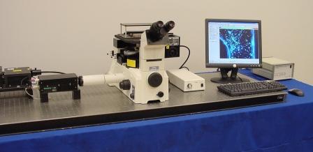
We used a TSI 1.4MP Peltier-cooled camera attached to a Nikon inverted microscope. A Big Sky 120 mJ Nd:YAG laser was used as the light source, however only a fraction of the maximum energy was used. The seed particles were 1 micron fluorescent dye PSL particles in distilled water.
The idea behind microPIV is similar to regular PIV in most respects, except that instead of using a light sheet to define the measurement plane, the entire volume of your measurement area is illuminated and the measurement plane is defined by the focusing plane of the microscope objective lens. The other main difference is that microPIV uses fluorescent particles as the tracers. These particles absorb the 532 nm light emitted from the YAG laser and emit light at a higher wavelength (around 560 nm). Within the microscope is an epifluorescent component that transmits the 532 nm laser light to the measurement region, but only allows the longer wavelength (fluoresced) light to make its way to the camera. Therefore, microPIV typically requires a very sensitive camera.
This is one of the image pairs obtained from the data. If your browser supports gif animations, the image is toggling between frame A and frame B. To make it stop, click your browsers "stop" button (click the image to see it full size). The time between laser pulses (delta T) was 50 microseconds. The flow direction is from top to bottom. Notice that since the magnification is quite high (0.16 microns/pixel), the particles appear fairly large. In addition, there really aren't that many particles in the frame compared to standard PIV. For this reason, and since this is a steady flow, it is common to use ensemble average correlation of the image pairs, in order to get good results. Ensemble averaging can be thought of as for any given interrogation region, summing the correlation maps across a set of images, effectively adding paticles to each interrogation region. It would be similar to adding the actual images together right on top of each other and performing the correlation on the resulting image. This provides for a much stronger correlation.
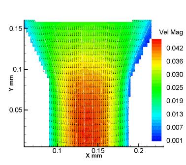
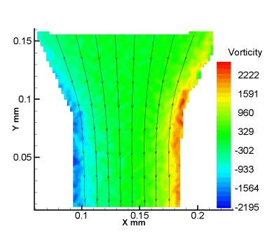
The following results are ensemble averaged over 50 image pairs. As you would expect, the velocity magnitude increases as the channel converges. The vorticity result indicates uniform shear layers on either side of the channel. Both plots suggest a symmetric parabolic velocity profile.